The Six-Signal Microstructure Cascade: How VisualHFT Instruments the Full Second Before the Print

Introduction

I have watched a market shift before the print moved. Not every time, and not with certainty, but often enough to build a monitoring stack around it. The pattern I kept seeing across desks in 20+ years of production HFT infrastructure was always sequential: cancel-side asymmetry first, then the book thinning, then VPIN climbing, then depth reshuffling across ten levels, then the spread widening, then the price print. One second, six signals, in roughly that order.

The question that consumed several years of instrumentation work was whether you could surface all six signals simultaneously, in real time, against a live feed, and render them in a way that a Head of Trading could act on. Not reconstruct post-close. Not read in a batch report. Watch them move, bar by bar.

That is what VisualHFT does. It instruments the cascade.

This article is the implementation companion to a neutral practitioner-research piece on the same cascade published at electronictradinghub.com. That version led with academic citations and gave VisualHFT a mention at the end. This version inverts the ratio: here the cascade is explained through the specific plugins and studies that render each signal live. The academic work sits underneath because it has to, but the organizing question is different. The question here is: which tile on your VisualHFT dashboard fires first, and what does it tell you before the book reflects it at the surface level?

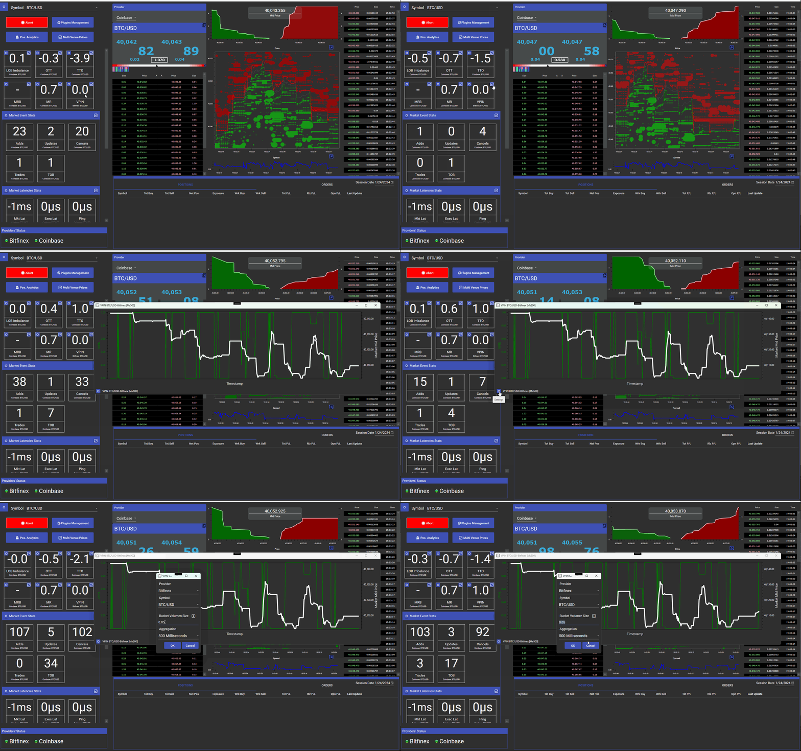
VisualHFT rendering full LOB depth against a live feed. Every level updates in real time. The cascade is not a theoretical construct; it is visible here, bar by bar, before the top-of-book spread reflects it.

The Cascade in One Second: Six Signals, Six Plugins

Before the section-by-section breakdown, here is the full sequence in one pass so the architecture is clear.

At T+0, the first signal is cancel-side asymmetry: cancels clustering three to five times heavier on one side of the book. This is a practitioner-calibrated threshold (not a canonical academic threshold), and it is the earliest visible signal in the sequence. The VisualHFT tile that renders this is the Order-to-Trade Ratio (OTR) tile, which surfaces the cancel-to-execution ratio per side in real time.

At T+10ms, the second signal is refresh-latency p95 widening: market makers slowing their quote replacement after each cancel. The VisualHFT metric is Market Resilience, which tracks how quickly the book reconstitutes depth after an aggressive order or a cancel sweep.

At T+50ms, the third signal is VPIN sustained above a practitioner-calibrated threshold (0.7 for 8 or more consecutive volume bars, in our implementation). Informed order flow concentration building before the price moves. The VisualHFT study is the VPIN Study, computed on a volume clock rather than a wall clock.

At T+100ms, the fourth signal is a structural shift across 10 or more depth levels of the LOB. The repositioning is no longer isolated to the top of the book. The VisualHFT plugin is the LOB Imbalance plugin, which renders bid-ask volume imbalance across the full available depth.

At T+500ms, the fifth signal is spread widening at the top of the book. By this point, the earlier signals have already told you the story. The spread reflects the cost of what the book already showed you.

At T+1s, the print moves.

The card that closes the companion LinkedIn video states this plainly: the full second is your lead time, if you are watching the book. The VisualHFT plugin architecture is built around that premise.

T+0 Cancel-Side Asymmetry: The OTR Tile

The earliest signal in the cascade is not price. It is not spread. It is the pattern of who is cancelling, and from which side.

Foucault, Hombert, and Roşu (2016, “News Trading and Speed,” Journal of Finance 71(1):335-382) formalized the mechanism: fast informed traders place limit orders ahead of news, wait, then cancel and resubmit aggressively when information materializes. The cancel is strategic. It precedes the commitment, not the other way around. Hendershott and Riordan (2013, “Algorithmic Trading and the Market for Liquidity,” Journal of Financial and Quantitative Analysis 48:1001-1024) confirmed that algorithmic traders contribute disproportionately to price discovery through exactly this pattern of cancel-and-reposition.

More recently, Dahlström, Hagströmer, and Nordén (2024, “The Determinants of Limit Order Cancellations,” Financial Review 59:181-201) decomposed limit order cancellations into motivated (strategic repositioning on new information) and mechanical (routine parameter-driven refresh) components. The key finding for practitioners: motivated cancellations cluster in time and are asymmetric by side. Mechanical cancellations do not cluster and are broadly symmetric. A sudden asymmetric cancel pattern on one side of the book, sustained across consecutive volume bars, is the empirical fingerprint of motivated repositioning.

The monitoring gap is that almost every standard dashboard tracks total cancellation volume, not side-level asymmetry. A book running 20% heavier bid-side cancels in a normal session will spike to 70-80% bid-side in the 30 seconds before an informed move. The daily aggregate smooths it to 22% and the signal disappears.

The VisualHFT OTR tile (Order-to-Trade Ratio) surfaces the cancel-to-execution ratio segmented by side. When the bid-side cancel rate diverges from the ask-side cancel rate by a sustained margin (in my practitioner experience, a three-to-five times asymmetry across consecutive bars is a meaningful signal, though this threshold requires calibration per instrument and venue), the OTR tile shows it in real time against the live feed.

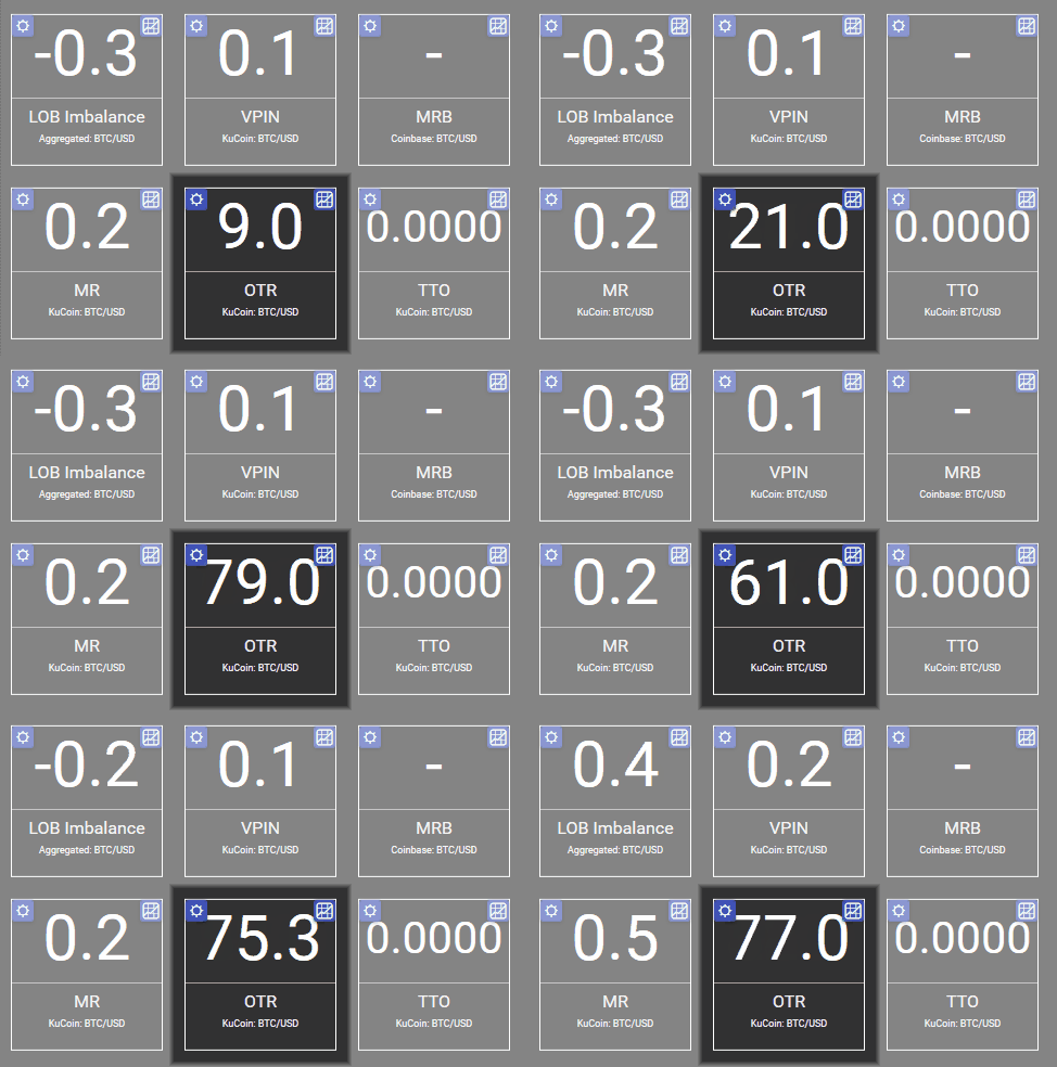
The OTR tile in motion. Cancel-to-execution ratio updating by side. The asymmetry that the daily aggregate smooths is visible here as it develops, before the spread number on the screen changes.

For the full cancel-side decomposition including regime diagnostics, the companion posts at Watching Cancel-to-Trade Ratio Drift in Real Time and Decoding the Cancellation-to-Trade Ratio cover the academic and regulatory context in more depth.

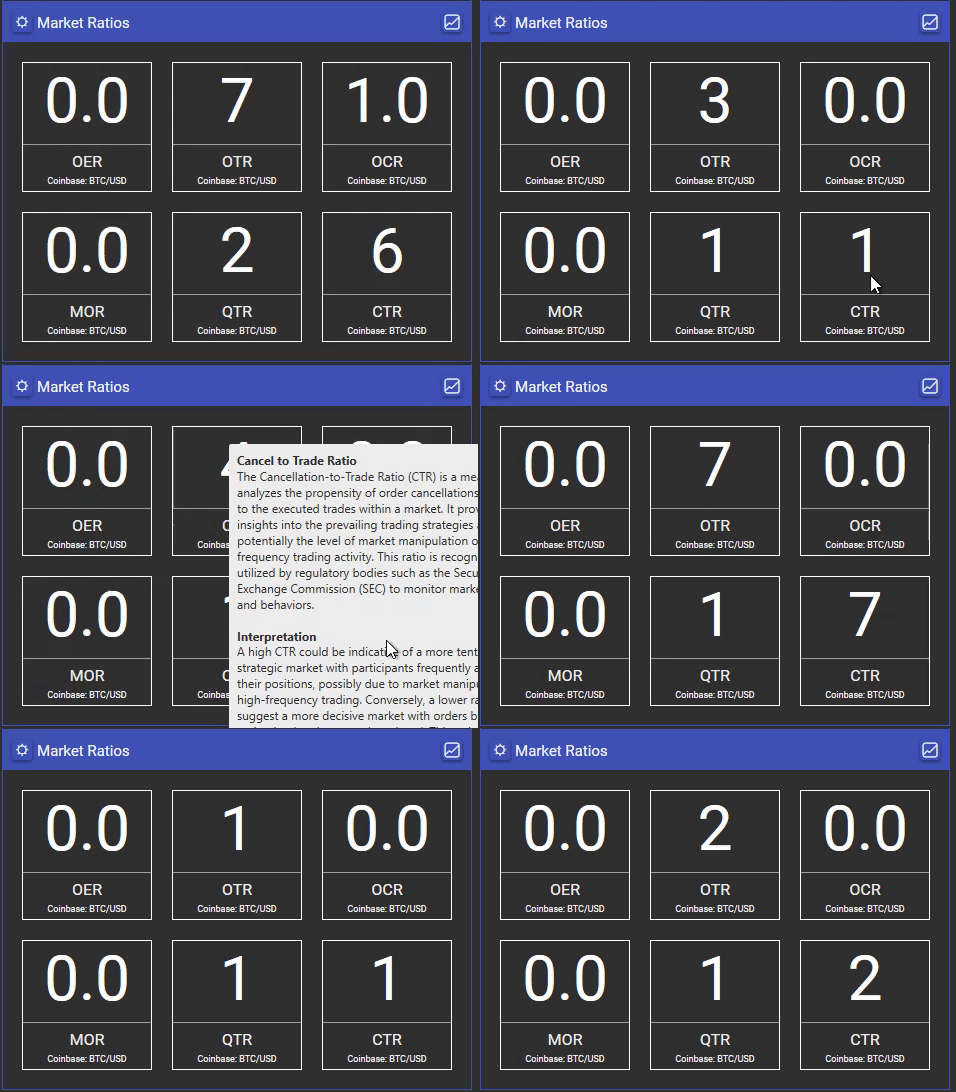
CTR animation showing asymmetric clustering on the bid side. Same session. The intraday spike that the daily file smooths is the signal worth watching.

T+10ms Refresh-Latency P95: The Market Resilience Metric

The second signal in the cascade is harder to see than the cancel count because it requires tracking the interval between events, not just the events themselves.

Bouchaud, Gefen, Potters, and Wyart (2004, “Fluctuations and Response in Financial Markets,” Quantitative Finance 4(2):176-190) established the conceptual foundation: the order book is a responsive system, and its response time is itself informative. Under normal conditions, market makers reconstitute depth quickly after disturbance. The response function of the book is tight. Under adverse selection pressure, the response function lengthens. Dealers are recalibrating before they recommit.

The practitioner translation: when market makers are comfortable, a cancel-and-requote cycle takes milliseconds. When they are not comfortable, that cycle slows. The p95 of the refresh-latency distribution widens before the mean does, because the cautious makers slow down first while the mechanical refreshers continue at normal cadence. The mean catches up only when the cautious fraction reaches a critical mass.

This is why monitoring the distribution, specifically the p95, surfaces the signal earlier than monitoring the average. A 10ms p95 widening to 40ms is a meaningful compositional shift in who is still providing liquidity and who has stepped back to re-evaluate. By the time the average crosses a threshold, the structural change has already happened.

The VisualHFT Market Resilience metric tracks how quickly the book reconstitutes after an aggressive order or a cancel sweep. The metric is a practitioner observation from production instrumentation, not a canonical published measure. But the underlying logic is directly grounded in the Bouchaud et al. response-function framework. When the resilience metric begins to degrade, the book is responding more slowly to disturbance than it was ten minutes ago.

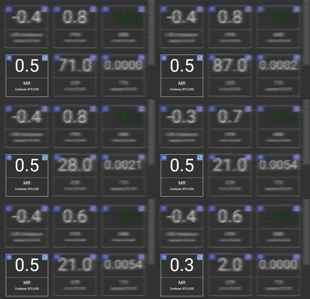
Market Resilience in motion. When the reconstitution rate slows, the book is responding more slowly to each cancel sweep. The p95 widens before the spread number changes.

The market resilience animation shows the same dynamic in stylized form, useful for pattern orientation:

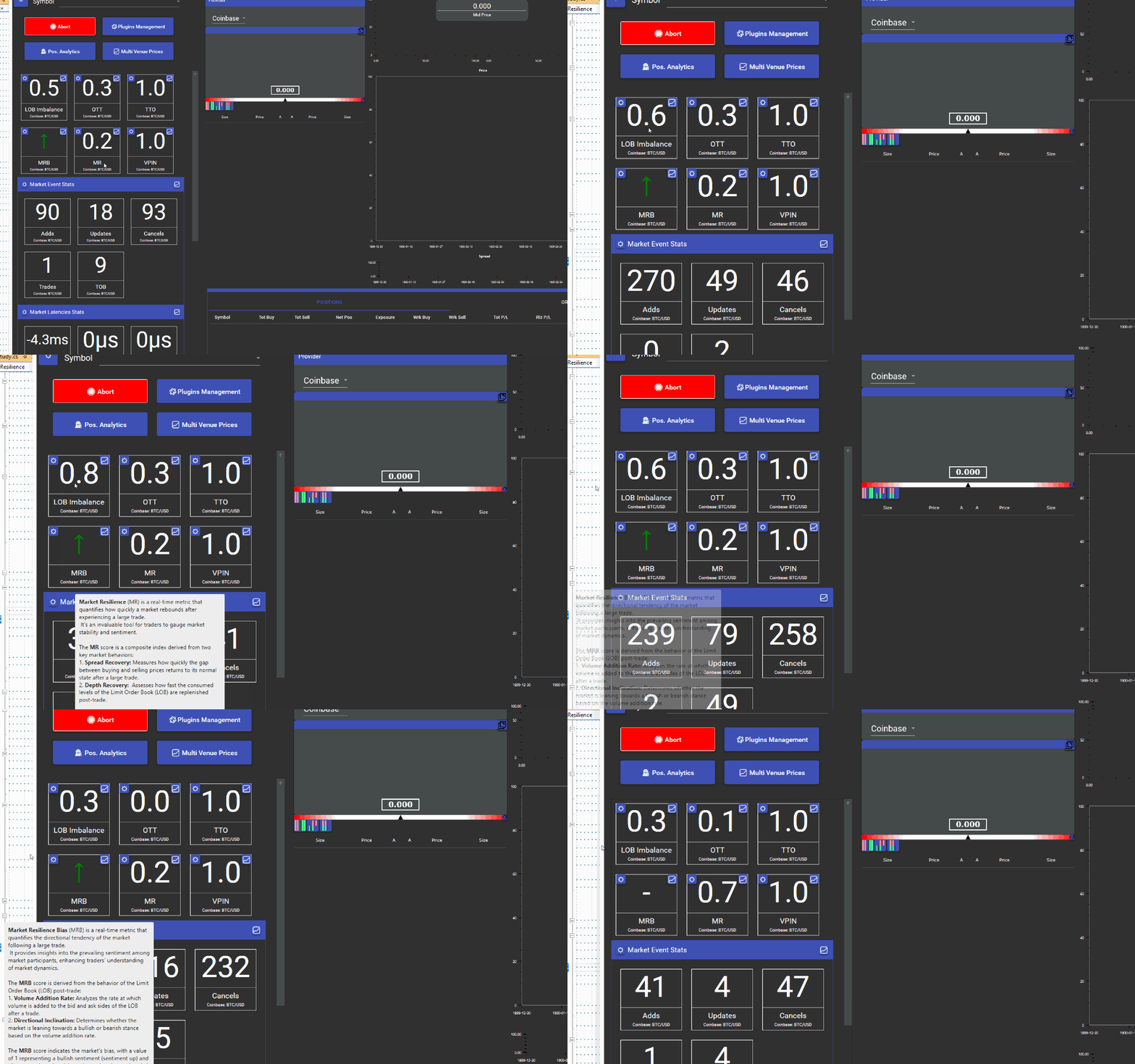
Stylized market resilience degradation. The slope of the reconstitution curve is the signal: steeper is healthier, flatter is market makers stepping back.

T+50ms VPIN: Volume-Clock Toxicity

The third signal is the one with the most academic coverage, the most debate, and the most implementation nuance.

Easley, López de Prado, and O’Hara published the foundational VPIN paper in 2011 (“The Microstructure of the ‘Flash Crash,’” Journal of Portfolio Management 37(2):118-128, using the event as a dataset, not as a narrative example) and the canonical VPIN framework in 2012 (“Flow Toxicity and Liquidity in a High-Frequency World,” Review of Financial Studies 25(5):1457-1493). The core mechanism: by segmenting volume into buy-initiated and sell-initiated buckets on a volume clock rather than a wall clock, you get a real-time updating measure of the proportion of informed order flow in the market. When VPIN rises, the composition of order flow has shifted toward informed participants.

The counter-evidence matters and should not be dismissed. Andersen and Bondarenko (2014, “VPIN and the Flash Crash,” Journal of Financial Markets) found that VPIN peaked after the event rather than before it, and that VPIN showed no incremental predictive power for future volatility once trading intensity was controlled for. That is a legitimate empirical finding on a specific event, and any implementation that claims VPIN is a reliable crisis predictor is overstating the literature. More recently, a 2026 study in Research in International Business and Finance (Vol. 81) extended VPIN analysis to Bitcoin markets, with findings relevant to crypto-native desks (we avoid specific statistics here due to paywall access constraints on the full paper).

The practitioner takeaway from the VPIN debate is narrower than the academic one: for execution quality monitoring, the question is not whether VPIN predicts discrete volatility events. The question is whether sustained elevated VPIN reflects a shift in order flow composition that affects fill quality. At sustained elevated readings, informed participants are concentrating activity. Market makers facing that composition widen spreads or pull depth. Your TWAP or passive posting strategy is being filled into a changed environment whether VPIN leads the price print by 30 seconds or moves simultaneously with it.

Two implementation decisions in VisualHFT’s VPIN Study are worth naming explicitly because they deviate from naive implementations and affect the metric’s behavior.

First, VisualHFT computes VPIN on a volume clock, not a wall clock. This matters in practice because volume clustering is a structural feature of electronic markets, particularly around news releases and opening/closing periods. A wall-clock implementation treats a high-volume minute as equivalent to a low-volume minute. A volume-clock implementation calibrates bucket size by traded volume, which keeps the VPIN estimate stationary with respect to the market’s own activity rhythm. The Easley et al. 2012 framework specifies volume-clock bucketing for this reason.

Second, VisualHFT uses BV-VPIN (bulk-volume classification) rather than trade-rule classification. BV-VPIN classifies the buy-sell split of each volume bucket using the price movement within the bucket rather than applying a Lee-Ready tick-test to each individual trade. Andersen and Bondarenko (2014) showed that BV-VPIN and TR-VPIN can diverge in specific conditions, which is a known limitation. For production monitoring, BV-VPIN’s computational tractability and its natural alignment with exchange-level data make it the operationally practical choice.

The threshold parameters in our implementation (0.7 as the sustained-elevation cutoff, 8 consecutive volume bars as the duration criterion) are practitioner-calibrated against the instruments we monitor. The Easley et al. framework used percentile-based thresholds (approximately the 90th percentile of the VPIN distribution, calibrated at roughly 50 volume buckets per trading day) rather than a fixed threshold. Any production deployment needs to derive its own thresholds from its own instrument data. The 0.7 and 8-bar figures are our calibrated values, not academic standards.

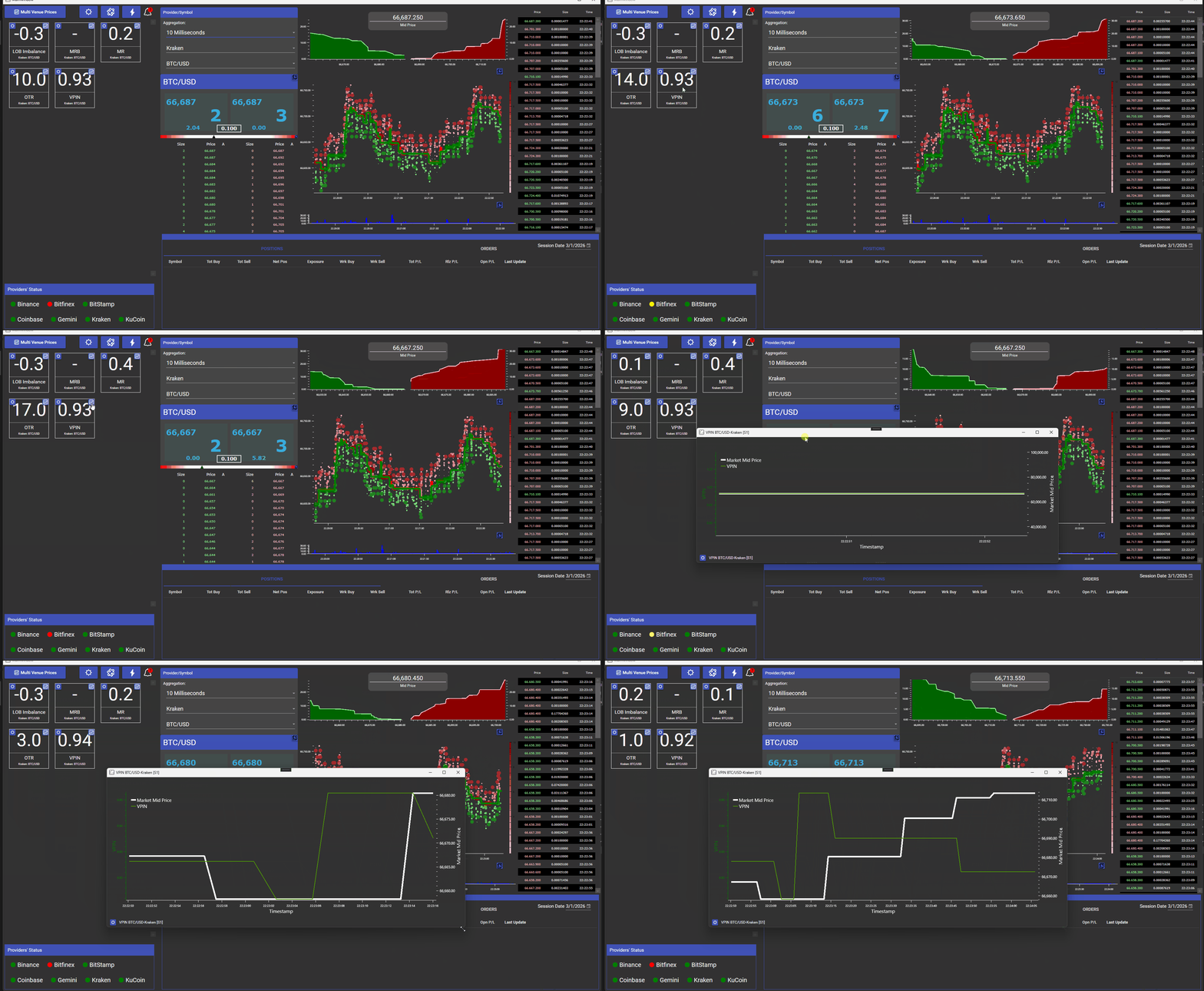
VisualHFT VPIN Study in motion. The metric updates on the volume clock, not the wall clock. Sustained elevation above the practitioner-calibrated threshold (0.7 for 8 or more consecutive bars in our implementation) is the condition that changes execution posture.

For the full VPIN implementation context, the companion articles at VPIN and Real-Time Order Toxicity and Volume-Synchronized Probability of Informed Trading: VPIN cover the academic debate and the monitoring stack architecture in more detail.

T+100ms Multi-Level LOB Shift: The LOB Imbalance Plugin

At T+100ms into the cascade, the informed repositioning that began as cancel-side asymmetry at T+0 has now propagated through the depth of the book. The signal is no longer visible only at the top. It is visible across ten or more depth levels.

Cont, Kukanov, and Stoikov (2014, “The Price Impact of Order Book Events,” Journal of Financial Econometrics 12(1):47-88) established the foundational relationship between order flow imbalance at the best bid and ask (level 1) and short-horizon price changes, with a linear relationship and a slope inversely proportional to market depth. This is the canonical reference for top-of-book OFI as a price predictor.

The critical extension for practitioners is Xu, Gould, and Howison (2019, “Multi-Level Order-Flow Imbalance in a Limit Order Book,” arXiv:1907.06230): they showed that extending OFI measurement to 10 or more depth levels materially improves short-horizon price prediction compared to level-1 OFI alone. The information content of the book is not concentrated at the top. Informed participants, particularly those who understand that top-of-book orders are more visible to adverse selection detection systems, often position their depth changes two, three, or five levels away from the best bid and ask.

What this means for monitoring: if your imbalance monitoring only covers the top of the book, you are reading the last sentence of the paragraph. The structural shift that precedes a price move is often visible as a coordinated repositioning across multiple depth levels, and it is frequently preceded by the cancellation patterns and VPIN elevation already described.

The VisualHFT LOB Imbalance plugin renders bid-ask volume imbalance across the full available depth, not just the top of the book. The plugin computes per-level imbalance and aggregates across depth, surfacing the directional pressure that is building in the structure of the book before it is visible in the spread.

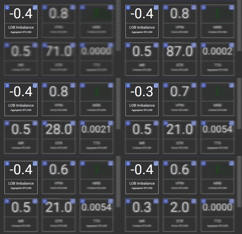
LOB Imbalance plugin in motion. Bid-ask volume imbalance updating across depth levels. The multi-level signal captures what top-of-book monitoring misses: structural directional pressure building two to five levels down.

The full LOB depth view (the hero image at the top of this article) shows the same dynamics from the full-book perspective: when the book reshuffles across depth levels, the movement is visible in the aggregate depth visualization before the top-of-book spread reflects the change.

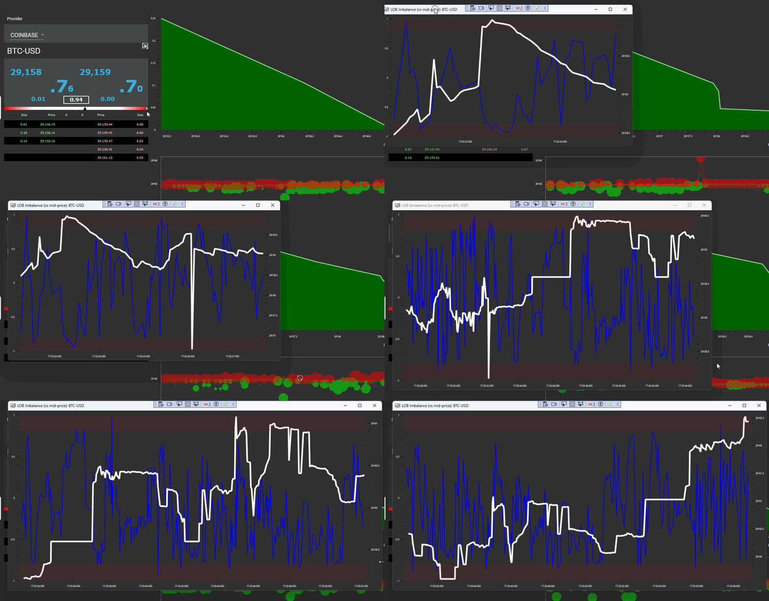
Secondary LOB imbalance animation. The directional pressure visible here is the same structural shift that the Xu/Gould/Howison 2019 multi-level OFI framework formalizes: extending measurement to 10+ levels improves price prediction compared to top-of-book alone.

For the deeper research context on LOB imbalances as a trading signal, the companion article at Leveraging Limit Order Book Imbalances for Profitable Trading covers the foundational papers and the monitoring architecture in more detail.

T+500ms Spread Widening and T+1s Print: Confirmation, Not Lead

The fifth and sixth signals in the cascade are the ones that most monitoring dashboards surface exclusively. The irony is that by the time the spread widens visibly at the top of the book, four earlier signals have already told you the story.

Glosten and Milgrom (1985, “Bid, Ask and Transaction Prices in a Specialist Market with Heterogeneously Informed Traders,” Journal of Financial Economics 14(1):71-100) formalized the mechanism: dealers widen spreads to recover the costs of trading against informed participants. The spread is not a cause of the cascade. It is the dealer’s accounting response to the adverse selection risk that the earlier signals already revealed.

Kyle (1985, “Continuous Auctions and Insider Trading,” Econometrica 53(6):1315-1335) introduced the lambda measure of price impact per unit of order flow. As informed participants concentrate activity, the market’s price-impact sensitivity rises. Kyle lambda is a structural consequence of the order flow composition shift that VPIN captures directly.

Moallemi and Yuan (2016, “A Model for Queue Position Valuation in a Limit Order Book,” SSRN 2996221) quantified queue position value at approximately the half-spread for some large tick-size stocks, not the full bid-ask spread. This is worth flagging because the queue position value literature is often cited with inflated figures; the half-spread finding is specific to large tick-size stocks and should not be generalized to other contexts.

The operational implication of the Glosten-Milgrom framework for VisualHFT users is straightforward: VisualHFT instruments the signals that precede spread widening, not the widening itself. The OTR tile, the Market Resilience metric, the VPIN study, and the LOB Imbalance plugin all fire earlier in the sequence than the top-of-book spread does. By the time your spread monitor alerts, the trade that informed participants are executing is already partially filled.

The price print at T+1s is not a signal. It is the settlement of a process that began one second ago in the cancel pattern. If your monitoring architecture alerts on the print, you are documenting the history of an event, not responding to its precursors.

The Multi-Venue Calibration Problem: VisualHFT Roadmap Open

Here is one thing I have not closed the loop on, and the community should know about it.

The cascade described here, from T+0 to T+1s, was calibrated on single-venue equities. The thresholds (three to five times cancel asymmetry, 0.7 VPIN for 8 bars, 10 or more depth levels) were derived from production experience on lit equity venues. They are not portable, without recalibration, to futures, crypto spot, dark pools, or alternative matching venues.

This matters for a few reasons. The microstructure of a CME futures book differs structurally from a Nasdaq lit book: tick size, fee structure, participant composition, and the relative size of the informed-to-uninformed trader fraction all shift the thresholds. A VPIN threshold that works on liquid equities may produce too many false positives on crypto spot, where the volume clock bucketing interacts differently with BV-VPIN classification during stress. The cancel-asymmetry signature may look different on a continuous-trading crypto venue than on a US equity market with circuit breakers and auction mechanisms.

The VisualHFT Multi-Venue plugin layout is built for per-venue instrumentation. Each venue runs its own plugin instance with independently calibrated thresholds. The architecture supports the “venue-class first, then aggregate” principle.

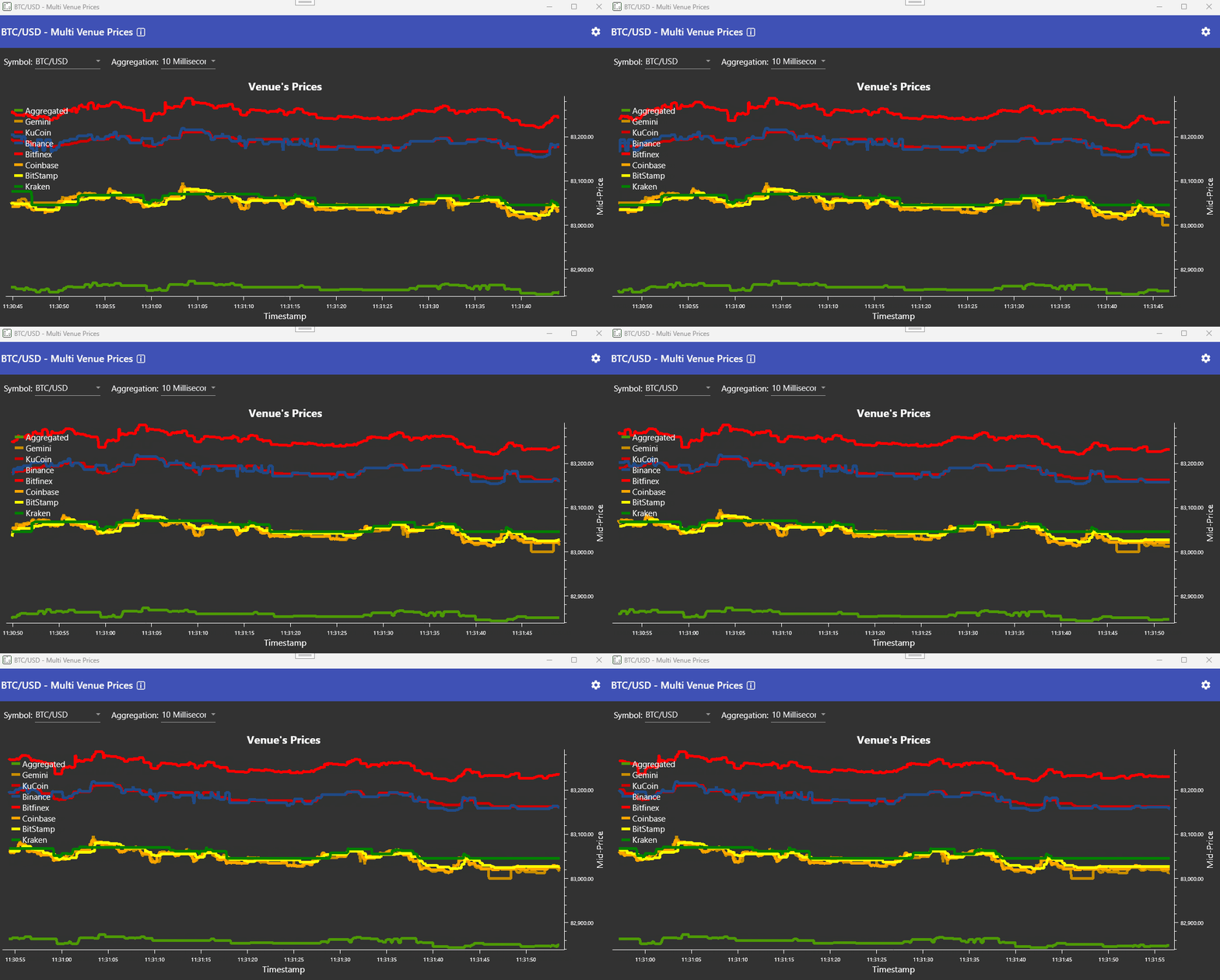
Multi-venue plugin layout in motion. Each venue runs its own data stream. Cross-venue calibration of the cascade thresholds is the open problem.

What the repository does not yet have is a validated cross-venue calibration framework. If you have instrumented the cascade on a futures or crypto venue and derived different threshold parameters, the methodology discussion in that PR or GitHub issue is the conversation worth having. The single-venue equity calibration is a starting point, not a finished product.

This is also the relevant caveat for DEX protocol teams: the cascade logic generalizes conceptually, but the latency regime and order flow composition of on-chain execution differs fundamentally from off-chain continuous matching. The plugins exist, but the calibration is on you and on the community.

The Diagnostic Protocol: What VisualHFT Surfaces vs. What Is on You

The question that follows from any monitoring stack is: what do you do with the signals?

The most productive framing I have found is the walk-back falsifiability test. Take ten fills from sessions where execution quality degraded. Walk each one back one second in VisualHFT. Which of the six signals fired before the fill? Was the OTR tile showing cancel asymmetry? Was the Market Resilience metric degraded? Was VPIN above the calibrated threshold? Was the LOB Imbalance plugin showing directional pressure across depth?

If the signals fired and the execution algorithm did not respond, you have identified an algorithm-signal feedback gap. The monitoring is working. The execution parameterization is not connected to it.

If the signals did not fire, the scenario falls into one of three categories. First, the event was genuinely outside the cascade pattern, which happens with large news releases that move price instantaneously without a preceding detectable order-flow buildup. Second, the thresholds are too conservative for the specific instrument and the signal was present but did not cross the alert level. Third, the data feed resolution is insufficient to capture the T+0 to T+50ms part of the cascade, in which case the monitoring gap is infrastructure, not algorithm logic.

The walk-back test is falsifiable because it produces a concrete answer per fill: signal fired or signal did not fire. That answer drives a specific remediation path in each case. It does not tell you whether the signal, if connected to the algorithm, would have improved execution quality on a risk-adjusted basis. That is the next test, which requires a controlled comparison across a meaningful number of fills.

VisualHFT surfaces what it surfaces: the six signals, in real time, against the live feed, with every computation traceable to the plugin source code. The threshold calibration is on the user. The connection to execution algorithm parameterization is on the user. The walk-back methodology is a starting point; the production validation is a longer process.

What VisualHFT does not do is tell you how to trade on the signals. That is a strategy problem, not a monitoring problem, and the architecture is deliberately designed to separate them. The plugin system surfaces microstructure state; the user decides what to do with it.

The VisualHFT architecture overview puts the separation in structural terms:

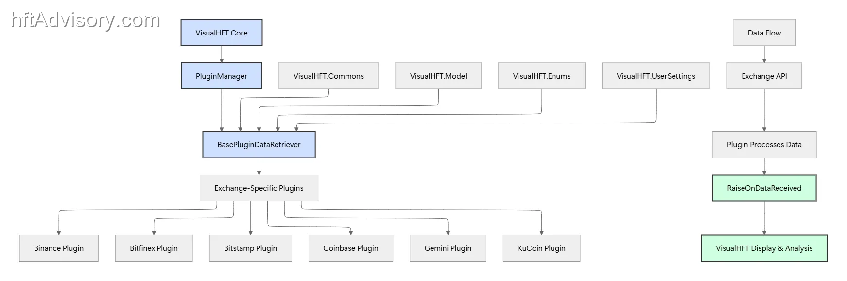
Architecture overview. The plugin separation between data layer, study layer, and rendering layer is intentional: monitoring microstructure state and trading on it are different problems. VisualHFT owns the first problem.

The study SDK flow makes the same point in implementation terms:

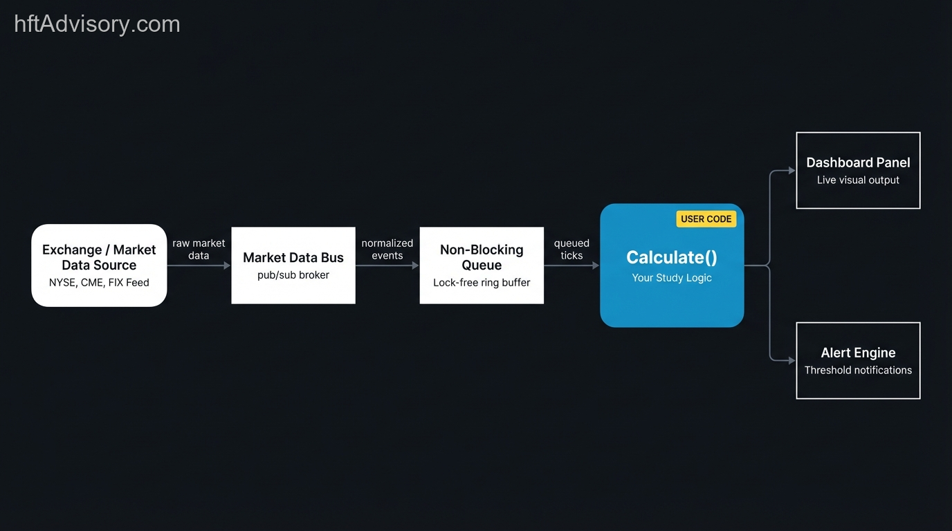
Study SDK flow. Every metric is an independently auditable plugin module. When VPIN spikes, you trace exactly what it is computing: the bucket size, the volume clock calibration, the BV-VPIN classification logic.

The open-source, over 1,000 GitHub stars repository is at github.com/visualHFT/VisualHFT. Apache 2.0, plugin architecture, and eight exchange connectors in the current build.

If you have run the walk-back test on your own fills and found a systematic pattern between signal firing and execution quality degradation, or a systematic absence of signal in cases where you expected one, that comparison is the contribution that advances the calibration framework beyond single-venue equities. The venue, the instrument class, and the threshold parameters you derived from your data are the variables that the community needs to converge on.

---

Originally shared as a LinkedIn post with a 60-second video walking through the cascade signal by signal. The same content also appears in practitioner-research form on electronictradinghub.com.

References

1. Foucault, T., Hombert, J., & Roşu, I. (2016). “News Trading and Speed.” Journal of Finance, 71(1), 335-382.
2. Hendershott, T., & Riordan, R. (2013). “Algorithmic Trading and the Market for Liquidity.” Journal of Financial and Quantitative Analysis, 48, 1001-1024.
3. Dahlström, P., Hagströmer, B., & Nordén, L. (2024). “The Determinants of Limit Order Cancellations.” Financial Review, 59, 181-201.
4. Bouchaud, J.-P., Gefen, Y., Potters, M., & Wyart, M. (2004). “Fluctuations and Response in Financial Markets.” Quantitative Finance, 4(2), 176-190.
5. Easley, D., López de Prado, M., & O’Hara, M. (2011). “The Microstructure of the ‘Flash Crash.’” Journal of Portfolio Management, 37(2), 118-128.
6. Easley, D., López de Prado, M., & O’Hara, M. (2012). “Flow Toxicity and Liquidity in a High-Frequency World.” Review of Financial Studies, 25(5), 1457-1493.
7. Andersen, T. G., & Bondarenko, O. (2014). “VPIN and the Flash Crash.” Journal of Financial Markets, 17, 1-46.
8. Cont, R., Kukanov, A., & Stoikov, S. (2014). “The Price Impact of Order Book Events.” Journal of Financial Econometrics, 12(1), 47-88.
9. Xu, K., Gould, M. D., & Howison, S. (2019). “Multi-Level Order-Flow Imbalance in a Limit Order Book.” arXiv:1907.06230.
10. Glosten, L. R., & Milgrom, P. R. (1985). “Bid, Ask and Transaction Prices in a Specialist Market with Heterogeneously Informed Traders.” Journal of Financial Economics, 14(1), 71-100.
11. Kyle, A. S. (1985). “Continuous Auctions and Insider Trading.” Econometrica, 53(6), 1315-1335.
12. Moallemi, C. C., & Yuan, M. (2016). “A Model for Queue Position Valuation in a Limit Order Book.” SSRN 2996221.